This post is a part of the series Advanced SQL Queries Via Practical Examples. You might want to go over the introduction first where I explain about the context. I use AdventureWorks2017 database in SQL Server for demonstration. You can download the database for free from the link above.
One of the main concerns when managing a business is tracking the effectiveness of sales activities. Performance indicators regarding sales include (but not limited to):
- Sales growth: How much have we sold ? Is our business growing steadily?
- Sales target: Are you on track regarding the sales targets?
- Revenues per sales rep: How much revenue do your sales rep bring?
As developer, our job is first to understand the questions so as to come up with solutions with data and technologies at hand.
In this post we will learn about fundamentals of window functions and how to use them to measure sales KPI. We will also take into consideration the performance drawback of window function and demonstrate an easy way to circumvent it.
We use the table Sales.SalesOrderHeader from AdventureWorks2017 database for our examples in this post. The table contains all orders made from 2011 to 2014 of Adventure Works bike company.
Now let’s approach some of very common questions using SQL queries.
Hightlights
“How much have we sold so far?”
We are likely to have heard this question many times over. “So far” reveals the demand for some kind of continuation from the past up until present. You would typically want to ask “Since when” to get more information. But in this case as let’s just go as far as we can all the way back to the very first order made in 2011 to the last one from 2014. We will calculate cumulative sales revenues of our bike company over 4 consecutive years using window function.
Using window function
Let’s first write this sub-optimized query to do what we want to do.
USE AdventureWorks2017
GO
SELECT DISTINCT
YEAR(OrderDate) AS 'YEAR',
SUM(TotalDue) OVER (PARTITION BY YEAR(OrderDate)) as 'SALES',
SUM(TotalDue) OVER (ORDER BY MONTH(OrderDate)) AS 'CUMULATIVE SALES'
FROM Sales.SalesOrderHeader
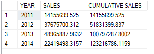
ORDER BY 'YEAR'What this SQL statement does is taking sales revenue from each year and adding it to the total of all previous years. For example, in line 3 we have the total of sales revenues from 2011, 2012 and 2013.
Overall result:
Notice OVER() clause that follows the aggregation operation? That is the part that defines a “window” for our SUM() function. A window is a subset of our dataset broken down either by time periods and/or by other criteria. These criteria are specified inside the OVER() clause. In the fifth line, as we write
SUM(TotalDue) OVER (PARTITION BY YEAR(OrderDate)) as 'SALES'we determine that our dataset is to be categorized by year, hence arranged into four segments, aka “partitions”. We use PARTITION BY to indicate the columns used to segregare our dataset. The SUM() is applied to each partition separately and computation restarts for each partition. This is the same as grouping data using GROUP BY then calculate sum for each individual group.
The difference between window function and GROUP BY is that grouping returns one row per unique group, while window functions, if not optimized, do the calculation per row and return all rows from the query. The GROUP BY therefore yields better performance because it discards intermediate results and returns less rows. Notice the DISTINCT in the query above is there to eliminate duplicates from returning results, which contain all 31,465 row from Sales.SalesOrderHeader table. This clumsiness results in severe performance problems. We will look more into this setback and how to improve our query at the end of this post.
Back to our sub optimized query, in the sixth line again we use window function to calculate running totals of sales revenues.
SUM(TotalDue) OVER (ORDER BY YEAR(OrderDate)) AS 'CUMULATIVE SALES'Without PARTITION BY clause, the function SUM() runs over all rows returned by the query, in this case the whole table Sales.SalesOrderHeader.
Even though our query returns the expected results, we can notice thousands of redundant rows and thus the need to use DISTINCT. The execution plan as well as I/O rates show that our query is doing horribly. The logical reads are twice the number of rows for each SUM() operation. This is due to the fact that window functions require intermediate results to be stored either in memory or on disk to do the aggregation. The number of intermediate results to store and where to store them depend on two factors: how the calculating frame is defined when processing each row, as well as the database engine optimizer. Based on high I/O rate, we know that SQL Server has chosen on-disk storage (I/O rate is high) for our query, and the reason for this is revealed later in the post.
Understand frame
We’ve seen that partitions determine individual bands to apply a window function, aka the absolute limits to restart calculations. Frame, on the other hand, defines how each row is processed and what to return for individual record. To better understand frame, we remove DISTINCT from our query and rerun it.
Overall result:
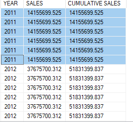
As you can see, in the third column results are accumulated year over year. However within a year, sales revenues are not accumulated per row, each row from the same year has the same "CUMULATIVE SALES" value. This is because our query didn’t specify partitions SQL infers one partition for the whole data set. Besides, when processing each row the window function must define the range of rows to include in the calculation, in this case any rows from the same year. This is what we call framing, or window frame.
RANGE vs. ROWS
If we don’t specify our framing, SQL Server define by default the frame by distinct values from the column(s) in ORDER BY clause. For example if we expand the ORDER BY expression:
SUM(TotalDue) OVER (ORDER BY YEAR(OrderDate), MONTH(OrderDate)) AS 'CUMULATIVE SALES'the frame is defined for each month of year. All rows within the same month and year will have the same returned value of 'CUMULATIVE SALES'. This is the default behavior in both SQL Server and OracleDB. In T-SQL the previous SUM() expression is the same as:
SUM(TotalDue) OVER (ORDER BY YEAR(OrderDate), MONTH(OrderDate)
RANGE UNBOUNDED PRECEDING)
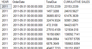
AS 'CUMULATIVE SALES'If this is the desired behavior and you want to add total from the start to the current row, you must change the argument from RANGE to ROWS (with an ‘s’). The frame therefore is defined for each row.
SELECT
	YEAR(OrderDate) AS 'YEAR',
	OrderDate,
	TotalDue,
	SUM(TotalDue) OVER (ORDER BY YEAR(OrderDate), MONTH(OrderDate)
		ROWS UNBOUNDED PRECEDING)
	AS 'CUMULATIVE SALES'
FROM Sales.SalesOrderHeader
ORDER BY YEAR, MONTH(OrderDate)
Overall result:
Now that we understood the fundamentals of window functions and window frame, let’s have some fun with more elaborate questions.
“How is our sales lately?”
This requires us get information about recent values and apply some sort of comparison in order to draw conclusions about performance. We can break the question into:
- What is the time frame ?
- What are the values that fall within this time frame ?
- How to compare these values with other periods ?
- Is our performance bettering or worsening ?
Moving averages
A proper answer for these questions above could be: finding out sales for the last three months, then calculating a performance indicator such as periodic average sales and sales share within a year to evaluate recent accomplishment, and finally gauging trends by computing moving averages.
SELECT
	YEAR(OrderDate) AS 'YEAR',
	MONTH(OrderDate) AS 'MONTH',
	SUM(TotalDue) 'REVENUE BY MONTH',
	AVG(SUM(TotalDue))
		OVER (ORDER BY YEAR(OrderDate), MONTH(OrderDate)
		ROWS BETWEEN 2 PRECEDING AND CURRENT ROW)
		AS 'MOVING AVERAGE REVENUE'
FROM Sales.SalesOrderHeader
GROUP BY YEAR(OrderDate), MONTH(OrderDate)
ORDER BY YEAR(OrderDate), MONTH(OrderDate)
The query groups sales by month and year so that we have each row monthly sales.
The SUM() function compute sales groups defined in GROUP BY expression. It makes up the input for the outer windows functions in the next expression.
The next expression calculates moving averages by taking into account current and two preceding rows. The frame is therefore three consecutive rows and it moves along the table. With ROWS options, we can easily calculate moving aggregation.
AVG(SUM(TotalDue))
		OVER (ORDER BY YEAR(OrderDate), MONTH(OrderDate)
		ROWS BETWEEN 2 PRECEDING AND CURRENT ROW)
		AS 'MOVING AVERAGE REVENUE'
Overall result:
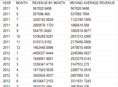
Moving aggregations, especially moving averages are widely used to sketch trends and forecast future values such as sales volumes, inventory levels, trading volumes or stock prices. Because of its popularity, it would be of great use to get acquainted with this technique.
The example above is rather simple just to demonstrate how easy it is to use window function. From business point of view, it is important to report per quarter and watch out for changes in growth rate. We can go further by adding more calculations such as sales percentage, average quarterly sales, quarter sales growth.
Growth rates
We may come up with a more complex query below, but let’s not be worry because I’ll break it down bit by bit.
WITH SALES AS
(SELECT
	YEAR,
	MONTH,
	QUARTER,
	SUM(TotalDue) 'REVENUE BY MONTH',
	AVG(SUM(TotalDue))
		OVER (ORDER BY YEAR, MONTH
		ROWS BETWEEN 2 PRECEDING AND CURRENT ROW)
		AS 'MOVING AVERAGE REVENUE'
FROM
	(SELECT
		YEAR(OrderDate) AS 'YEAR',
		MONTH(OrderDate) AS 'MONTH',
		CASE
			WHEN CAST(MONTH(OrderDate) as decimal) / 3 <= 1 THEN 1
			WHEN CAST(MONTH(OrderDate) as decimal) / 3 <= 2 AND CAST(MONTH(OrderDate) as decimal) > 1 THEN 2
			WHEN CAST(MONTH(OrderDate) as decimal) / 3 <= 3 AND CAST(MONTH(OrderDate) as decimal) > 2 THEN 3
			ELSE 4
			END AS 'QUARTER',
		TotalDue
		FROM Sales.SalesOrderHeader) innerquery
GROUP BY YEAR, QUARTER, MONTH),

SALES_QUARTER AS
(SELECT *,
	SUM([REVENUE BY MONTH])
		OVER (PARTITION BY YEAR, QUARTER  ORDER BY YEAR, QUARTER)
		AS 'TOTAL QUARTERLY',
	AVG([REVENUE BY MONTH])
		OVER (PARTITION BY YEAR, QUARTER ORDER BY YEAR, QUARTER)
		AS 'AVERAGE QUARTERLY',
	100*(SUM([REVENUE BY MONTH])
		OVER (PARTITION BY YEAR, QUARTER  ORDER BY YEAR, QUARTER))/(SUM([REVENUE BY MONTH]) OVER(ORDER BY YEAR)) AS 'QUARTER/YEAR PERCENTAGE'
FROM SALES)

SELECT
	100*([TOTAL QUARTERLY] - ((LAG([TOTAL QUARTERLY],1) OVER (PARTITION BY YEAR ORDER BY YEAR))))
	/(LAG([TOTAL QUARTERLY],1) OVER (PARTITION BY YEAR ORDER BY YEAR)) AS 'QUARTER GROWTH'
FROM SALES_QUARTER
ORDER BY YEAR, QUARTER
Our query is in fact composed of four sub queries, the innerquery just selects columns from our working table, does some transform and return us a proper data set to work on. Then we use common table expression to store result sets from the second and third queries in SALES and SALES_QUARTER. It’s just an readable way to organize subqueries.
SALES store results from calculations per month basis. SALES_QUARTER store results aggregated by quarter. And the outermost query at the end computes sales growth from quarter to quarter of the year. LAG() operator is very convenient to get value from the previous row.
LAG([TOTAL QUARTERLY],1) OVER (PARTITION BY YEAR ORDER BY YEAR)The expression above retrieves total quarter revenue from the previous row and restarts for each year. Then use it to calculate growth using simple formula 100 x (current amount - previous amount) / previous amount. We have this formula translated into SQL below
100*([TOTAL QUARTERLY] - ((LAG([TOTAL QUARTERLY],1) OVER (PARTITION BY YEAR ORDER BY YEAR))))
	/(LAG([TOTAL QUARTERLY],1) OVER (PARTITION BY YEAR ORDER BY YEAR)) AS 'QUARTER GROWTH'
Overall result:
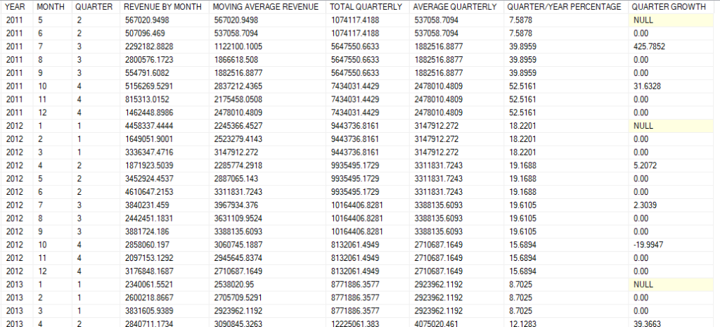
Column QUARTER GROWTH in figure 5 reads for example: sales in third quarter of 2011 grew 425.78% from second quarter. You can then use data from our query to create graphs in order to better visualize changes and trends, look for consistent patterns overtime and seek to understand sudden changes.
Window function performance consideration
You may notice that, if columns in ORDER BY clause contains only unique values, ROWS and RANGE will produce the same results. For example:
SET STATISTICS IO ON;
GO

--query1
SELECT
	YEAR(OrderDate) AS 'YEAR',
	SUM(TotalDue) OVER (ORDER BY YEAR(OrderDate)
	ROWS UNBOUNDED PRECEDING) AS 'CUMULATIVE SALES'
FROM Sales.SalesOrderHeader
ORDER BY YEAR

--query2
SELECT
	YEAR(OrderDate) AS 'YEAR',
	SUM(TotalDue) OVER (ORDER BY YEAR(OrderDate)
	RANGE UNBOUNDED PRECEDING) AS 'CUMULATIVE SALES'
FROM Sales.SalesOrderHeader
ORDER BY YEAR
Both queries will return the same result set because in the query2 the frame is defining over unique values from the column SalesOrderId, and it is the same as framming per row.
The difference between ROWS and RANGE in this case may be subtle, but there is a huge gap in performance and so it is worth to be inquisitive about this drawback and learn to optimize.
When running the query in SQL Server with SET STATISTIC IO ON, we can see a huge difference in the number of I/O reads between two queries. We have 64,837 logical reads reported for “Worktable” from the query2 and 0 for query1.
We have seen above that windows functions require intermediate results to be stored either in memory or on disk, more precisely in the “Worktable“. The number of logical reads greater than zero mean these results are potentially spilled to disk which causes high memory pressure or high disk I/O rate.
The reason for this is in SQL Server results are always stored on disk when the framing for window functions is RANGE UNBOUNDED PRECEDING, or when number of rows to proceed exceed 10000 regardless of mode. When using ROWS mode with UNBOUNDED PRECEDING, SQL Server knows to store only the result from previous rows and the detail for the current row. Framing by RANGE is therefore much slower and very costly in comparison with ROWS. Use RANGE only if you want to include all rows from the same group in the aggregation and always have the same result regardless of row’s position.
We’ve seen that when processing large table, window functions introduce some performance overhead. So does it mean we should abandon window functions altogether ? There are ways to reduce alleviate this problem while taking full advantage of window functions.
Optimization
Pre-aggregation
One way to minimize the performance hit by window functions is pre-aggregate our data set using GROUP BY so as to apply window function only on a small set of results. We’ve seen this technique above to calculate average and total sales per quarter. When look into the statistics, our complex query actually has very good performance, only 260 reads reported from “WorkTable”.
Back to our sub optimized query on top of the post, we can improve it by grouping our data first and apply window functions on top.
USE AdventureWorks2017
GO
SELECT
	YEAR(OrderDate) AS 'YEAR',
	SUM(TotalDue) as 'SALES',
	SUM(SUM(TotalDue)) OVER (ORDER BY YEAR(OrderDate)) AS 'CUMULATIVE SALES'
FROM Sales.SalesOrderHeader
GROUP BY YEAR(OrderDate)
ORDER BY 'YEAR'
Batch mode processing
Traditionally data is processed per row basis, this is the row mode. Batch mode is introduced since SQL Server 2012 to optimize processing workload for data warehouse, where data could excess billions of rows. In batch mode, SQL Server groups rows into batches to process.
Since SQL Server 2019, batch mode is enabled for aggregations on large table (millions to billions of rows) with database’s compatibility level of 150 or above. The same query on the same hardware runs at least 3 times faster with batch mode on. It is possible to turn on or off batch mode in SQL Server 2019:
--Check compatibility level
SELECT compatibility_level
FROM sys.databases WHERE name = 'AdventureWorks2017';
GO

-- Set compatibility level to 150 for batch mode to work with rowstore indexes
ALTER DATABASE AdventureWorks2017
SET COMPATIBILITY_LEVEL = 150;
GO

-- Turn on batch mode
ALTER DATABASE SCOPED CONFIGURATION SET BATCH_MODE_ON_ROWSTORE = ON;
Before SQL Server 2019, batch mode is enabled only on table with columnstore indexes. Therefore, to take advantage of batch mode processing creating columnstore indexes may also be an option if the table is not updated regularly.
In the next article we’ll learn to use window functions in combination with PIVOT to produce more interesting reporting tables.
Further readings
I have recently started a site, the info you provide on this web site has helped me greatly. Thanks for all of your time & work.